The Solution

Step 1. Decompose the image into small cells. Each grid contains 16*16 pixels.
Step 2. Compute the histogram in the RGB levels (All grid has three (red, green, blue) histograms.).
Step 3. Classification based on the correlation of histograms.

Step 4. Segment the image.

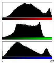
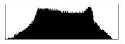
Solution 2. - Histogram matching II.

Differences from Histogram Matching I.
Convert the histograms to a greyscale. (Y=0,299 R+0,587 G+0,114 B)

• Statistics based classifier algorithm
• Uses spatial information
• Driven by energy minimization

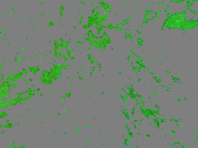
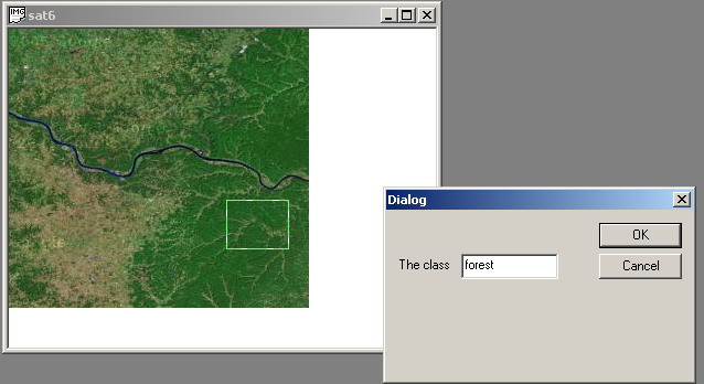
Solution 4. - Texture-based recognition 

     Features used:

•  average edge frequency (density)

                               D   =  no_of_edge_pixels/total_no_edge_pixels

• average edge contrast

                               E(d) =Sum_i,j(|f(i,j)-f(i+d,j)| + |f(i,j)-f(i,j+d)|+|f(i,j)-f(i-d,j)|+|f(i,j)-f(i,j-d)|)

•  GLCM

    C_D (g₁, g₂) =  #{((x,y), (x’,y’)): f(x,y)=g1, f(x’,y’)=g2, x=x’+dx_i y=y’+dy_i}

• GLCM (Gray Level Cooccurrence Matrix) homogeneity

•  GLCM (Gray Level Cooccurrence Matrix) entropy

            Entropy = - ∑∑  p(i, j)log p(i, j)   

  ^{i   j}

•  GLCM (Gray Level Cooccurrence Matrix) variance

Variance =  ∑∑ (i - μ)² p(i, j)   

               ^i  j

•  GLCM (Gray Level Cooccurrence Matrix) energy

            Total_energy= ∑∑ (p(i, j) )²   

                        i  j

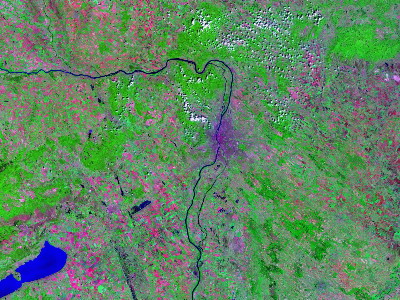
 Step 1. Learning

• Select a known region int the image (forest mountains or water)

• Compute GLCM features and edge-based features

• Store the feature vector in the training set for the corresponding class

 Step 2. Recognition

•  Select an unknown area in the image in order to classify it: forest mountains or water

• Compute  the GLCM features and the edge-based features

• Compare the feature vectors with the data int he training set: euclidean distance

• Use the k-nn method and decide the class